Welcome to the K0FC site

The Ham Radio Computer

The ARRL technical magazine QEX has published, on the July/August 2025 issue, an article describing my software HRC (Ham Radio Computer).

While I strongly recommend the reading of the QEX magazine (available on the ARRL site), you may download the HRC software and guide from the present website. Thank You for your interest in the HRC project.

What is the HRC?

How does it works?

Which instruments do I need?

Measuring an antenna tuner

Transmission lines

Does it worth to change the cable?

Parallel stub positioning and dimensioning

Coherence check

Power level comparison

The power meter limitations

Exit ways

Measuring impedance and voltage

Measuring current

Half... final considerations

Saving the best for last: VNA-only power comparison

NanoVna directions

An example of tuner comparison

Credits

What is the HRC?

The HRC, Ham Radio Computer, is a software developed by Claudio Facciolo, K0FC, for the ham radio community. It is available for free for Windows operative systems, and it can be downloaded from the following link: www.k0fc.net/content/files/HRC31.exe

The HRC can perform every impedence, voltage, current, power and SWR computation on tha antenna, on the transmission line and on the radio.
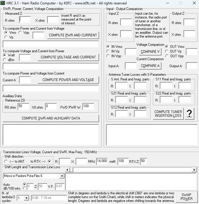
The software is divided in three sections, left, right and lower.

How does it work?

Let’s start from the left section.
Entering the two impedance values, R and X, you get power and current from voltage, or, you can enter power and get voltage and current. To close the loop, you can enter current and get power and voltage.
The lower window of the left section will show you the SWR and the additional data related to the impedance: return loss, reflected power, reflection coefficient (also called Gamma or S₁₁) real and imaginary parts, magnitude, phase and admittance.
The software computes these data using complex numbers algebra, since these values are formed by a real part and an imaginary one, which are subject to Ohm’s laws applied to impedance.
The complex numbers fits the need to completely represent the impedance values. While the real part of the complex number is the resistance R, the imaginary part is the reactance X.
Now an example.
We are going to choose a 4:1 balun.
Many manufacturers provide the maximum power the device can bear, but generally this power is related to a 200 ohm impedance, without reactance. Let’s see what our software will show. Please enter R = 200 and X = 0, then compute which voltage and which current we have with 100 watts:

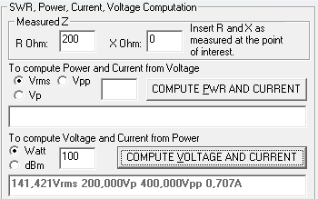
The voltage is slightly above 140 Vrms, 200 Vp or 400 PEP and current is 0,71A.
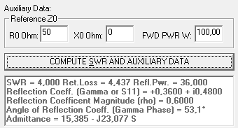
Now let’s enter R = 50 and X = 75.

While this time voltage has slightly decreased, the current has doubled, notwithstanding exactly the same SWR value, 4, as shown clicking on “Auxiliary Data”.

The HRC is a valid tool to properly verify the voltage and current values we will experience according to the different impedances we will deal with, avoiding to learn them in the hard way.

Which instruments do I need?

Unless you already know the values of the real and the imaginary impedance parts (resistance and reactance), you have to properly measure them. The VNA, or Vector Network Analyzer, is the dedicated instrument for this purpose. A well known version of the VNA, when equipped with a single port, is the so-called antenna analyzer. If we already have an antenna analyzer, we shall use it for the first examples, as we will need the two-ports version of the VNA for the advanced measurements methods that will follow. We could use a basic model, but we should know the limitations.
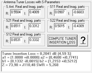
Many analyzers and VNA are based on the VSWR bridge. This method gives valuable results starting from 10 or 20 ohm to a few hundreds. In case we need to measure very high or very low impedances, an VSWR bridge based instrument will give less precise figures. Better would be to use the RF-IV method, where IV stands for current and voltage, which gives valuable results from very few ohm until thousands. A device that can adopt this feature, when used in conjunction with an external dedicated board and its own software, is the VNWA 3 by DG8SAQ.

Cheap analyzers do not show the reactance sign. For several measurements this is not a vital data. If you enter the wrong sign, voltage, current and power data will not be affected, but you will need to ignore several values in the Additional Data window.

Measuring an antenna tuner

The antenna tuner is a suitable device to be measured. This device couples very different impedance values, so it is important to determine the voltage and the current values involved in its components. If it is a relay-based automatic antenna tuner, this knowledge is of the utmost importance. Relays are generally the weak link in the tuner circuit. If, for instance, it is 300V PEP and 10A rated, and we want to determine the maximum power we can use not to overcome these ratings with a Z formed by R = 50 and X = 75, we shall enter the following data in the HRC:

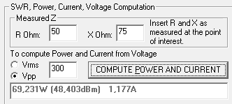
A 70W power already reaches the 300V PEP limitation, with a rather low SWR. Instead, an impedance formed by R = 20 and X = 40, that presents a slightly higher SWR value, will exceed the same voltage limitation with a 112,5W power.

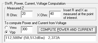
In both cases current is well below limits.
We will probably be able to measure impedance at the input and output ports of the tuner, but Z will be different inside. Nevertheless, the input and output values will give a solid idea of the stress the internal components will be subjected to.

Transmission lines

Another RF component we want to check is the transmission line. It is important to underline that a transmission line, whichever its characteristic impedance Z₀is, will always perform an impedance transformation when the antenna impedance is different from Z₀. So, the impedance along the line will vary to return “almost” to the initial values of Z₀, after a length corresponding to ½ wavelength. The line attenuation is of the utmost importance in determining the “almost”. Let’s now examine the lower HRC section, to explore what happens along a transmission line of whichever its nature or impedance, 50 or 75 ohm coaxial cable, or high impedance ladder line.
The first step is to enter the shift direction from our measuring point, both if we move from the antenna towards the RTX, or viceversa. Then we enter the R and X values as measured by our instrument, the line charateristic impedance, its velocity factor (V.F.), the operating frequency and the power (where we measure the impedance, later we will see how to enter the RTX power). Or, even simpler, we can leave the automatic mode and select one of the transmission line from the curtain menu. HRC will compute the impedance values, SWR (both respect to the line and to the RTX, if different), voltage, current and the shift expressed in degrees, wavelengths (electrical length), meters (phisycal length) and losses. The fourth row, as we will see later, reports parallel impedance and stub values.

To highlight that after ½ wavelength values almost repeat themselves, this measure becomes a sort of new unit of measurement. Nevertheless, you will have no difficulties in entering the shift length in meters or degrees.
Let’s see the reason why this recurrence is not perfect. When RF travels from the radio to the antenna, part of its power will be dissipated along the line. Should a mismatch be present, the reflection will take place on a lower level of power than that present at the radio. And this reflected power will be attenuated too, travelling towards the radio. So two attenuations are present, one affecting the direct power, and one affecting the reflected power. The result is an alteration of the ratio between the direct and the reflected power at the radio. That is, a different SWR value take place, always lower than if the line were were lossless. With the same SWR at the antenna, the higher is the attenuation, the lower will be the SWR at the radio.
We have to take in account another factor. Manufacturers declare the attenuation for a perfectly matched line (Matched Loss, or ML). Of course they do not know what the mismatch is in the different cases. But when a mismatch occurs, the RF travels forward and back along the line, so we experience an additional loss, which depends on the mismatch level.
There are tables to compute this additional loss, but you have to enter the SWR which is present at the antenna. There is no way to use these tables from the RTX end, when you know the radio SWR and not the antenna one. But again, no sweat. The HRC is able to compute the additional loss whichever is the shift direction, so you do not have to make any correction. As long as the SWR is less than 25, results are accurate and in accordance with the ARRL Antenna Book tables.
Now an example.
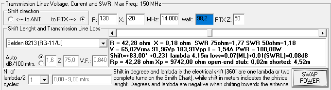
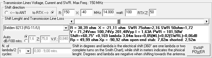
We have a monoelement Delta Loop for the 20 meters band. We check Z at the feeding point with an antenna analyzer, obtaining R = 130 and X = -20. We want to realize a 75 ohm stub with the Belden RG-11/U (8213) to lower the SWR as much as possible. The velocity factor of the coaxial cable stub is 0.67 and we plan to use 100W, while the RTX impedance is the standard 50 ohm. Let’s enter all these values on the HRC. This is the starting point we obtain by touching the cursor:

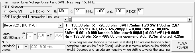
Since we measured the impedance right on the antenna, the shift direction to choose is obviously “to RTX”.
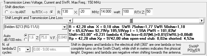
Shifting the cursor, data will be presented underneath. We will probably want the lowest possible SWR. We will find that a cable length of 4,15 meters satisfies this request.

I would like to point out that, moving the cursor, you will have the new values ready at hand. So it is easy to verify, for example, the maximum voltage and power values you will experience on the line. Just like a board game, every time you pass over the “Start” (the one half wavelength shift) the values are again similar to the initial ones. So every place in the transmission line has its own set of value, and you can go forward or rearward. It reminds me of the good old Monopoly®!

It is easy to verify that, in a one half wavelength space:

Reactance X is 0 always and only twice.
Where reactance is 0 you will obtain a maximum value voltage or a minimum value one.
Where a maximum value voltage is present, there you find a minimum value current, highest resistance, 0 reactance.
Where a maximum value current is present, there you find a minimum value voltage, lowest resistance, 0 reactance.

Let’s have a closer look to the power results: we input a 100W value, and the result is almost 102. This is something we expected: power on the RTX side is higher than on the antenna side. The cable length is very short, so this difference is not evident, still is present. The value we input is the power measured where we put the VNA to check the impedance, in order to have a topographic coherence. Maybe we are not able to measure the power level at that point, and so we prefer to take into account the power from the RTX. In this case just activate the Swap Power option: in the power window, on a blue blackground, a new number will be shown. It is the power you should have on the measured point in order to have the initial level on the computed point, in this case the RTX:

The Swap Power option can be activated on the “to ANT” shift too. In this case you can calculate the power necessary on the RTX in order to have a specific power level on the antenna.

Does it worth to change the cable?

Now another example:
We have 18,00 meters of generic RG-58 coming from the antenna. We measure the impedance at the RTX end. For a frequency of 21.000 MHz we have R = 100 and X = 70 ohm. SWR is 3,16 (you can double check with the upper left section with the Auxiliary Data). We want to compute the advantage, pertaining attenuation, swapping the cable with 18,00 meters of Messi e Paoloni Hyperflex 10. This is the starting point:

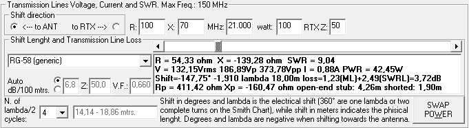
The computed impedance at the antenna is R = 54.33 and X = -139.28 ohm, SWR is more than 9. We lost 3,72 dB (mainly for mismatch) and the power reaching the antenna is 42,45 watt.
We now use the computed value with the shift in the opposite direction, towards the radio, and this is the result after power swapping:

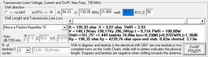
Now the power at the antenna is 74,2 watt, 30 watts more than with the RG-58, a 75% increase in relation to the 42,45 value. Of course the same 75% increase will be present on the received signal, too.
It is interesting to note that SWR has increased too. And it is exactly what we expected, due to the attenuation of the direct power towards the antenna and the reflected one towards the radio, diminishing the ratio between reflected and forward power.

Note: I would like to emphasize that all the three SWR values, 9,04 at the antenna, 3,16 after 18 meters of RG-58 and 3,93 after the same length of Hyperflex are all correct and coherent. The antenna has an SWR of 9,04 in respect to the 50 ohm cable impedance. The longer is the line, the more attenuated is the signal. And since attenuation is greater with the RG-58, the same length of this cable will produce more attenuation, lowering the SWR.

Parallel stub positioning and dimensioning

In case we would like to use the parallel stub method to cancel reactance and adjust resistance at the same time, to have a unitary SWR along the line, it will be necessary to determine the exact distance from the antenna where to connect the parallel stub, and, of course, to compute the stub length, either open-end or shorted-end.
Parallel impedance values, Rp and Xp, are shown on the fourth row. HRC computes the stub as if it is made of the same transmission line, or at least with the same velocity factor and characteristic impedance.

Let’s present an example.
We have an antenna with an impedance of Z = 150 - J40 at 14 MHz. We will look for a shift along the line (Messi e Paoloni Ultraflex 7) where the parallel resistance Rp is 50 ohm. The first point is located 2,73 meters after the antenna:

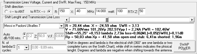
HRC says that at 2,73 meters from the antenna parallel resistance Rp is 50,03 ohm. If at this point we connect a 6,41 meters open terminated stub, or a 1,96 meters short terminated one, we will compensate for the reactance, but when reactance is canceled, the serial resistance is equal to the parallel resistance. So, from this connection point on, the impedance (both serial and parallel) will be 50 ohm without any reactance until the RTX.

When reactance is capacitive (Xp < 0), and this is the case, we can expect the shorter stub to be the short terminated one. When is inductive (Xp > 0), the shorter will be the open terminated one.
If we ignore this point at 2,73 meters, we will meet another point before the ½ lambda length where the Rp is 50 ohm:

In this case the reactance is inductive (Xp = 43,10 ohm), so the shorter stub is open terminated, the longer is the short terminated one.
Taking losses in consideration, it is advisable to choose a connection point as close to the antenna as possible, in order to reduce the transmission line length where SWR is present. Then we can choose between open or shorted-end stub.
Open stubs are easier to build and to adjust, while shorted stubs are more electrically solid and durable, since they are less sensitive to weather contaminations. HRC leaves to us the choice where to put the stub, in the usual way of shifting the cursor, so we can choose the most suitable point, since sometimes it is not feasible to use the closest point to the antenna.

It is also possible to connect a stub where the parallel resistance is different from the characteristic line impedance. In this case, impedance will vary after the connection point with the stub, unless we use a cable whose impedance is the same of the chosen value. Let’s make an example.

Same antenna as the previous one, on the same frequency. We have a remnant of Belden 8213 RG-11/U, about 20 feet. Let’s check if it we can use it for the initial part of a transmission line and to build a stub.
Since SWR is high enough, there are points where the parallel resistance is around 50 ohm on the 75 ohm line. The first is at 3,04 meter from the antenna:

At 3,04 meter from the antenna we have an Rp = 49,99 ohm, so we connect the RG-11/U cable with a 50 ohm impedance cable. At the same point, we connect in parallel a 2,52 m shorted-end stub to cancel the reactance (Xp = -90,92 ohm), made with the same RG-11/U cable (or another 75 ohm impedance cable, with the same velocity factor). From the connection point to the radio, the impedance will not vary anymore from the value of 50 ohm, without any reactance, obtaining an SWR of 1.

Computation confirmation and coherence check

Let’s now present a case where we can check the reliability and coherence of the HRC results.

Consider an antenna with an impedance of R = 150 and X = 0 at a frequency of 50 MHz. We know the SWR is 3 and that reflected power is exactly ¼ of the forward power. The transmission line is made of 30,48 meters (exactly 100 feet) of Belden RG-213 (8267). We want to compute the SWR at the RTX end of the cable. Before opening the HRC, let’s make some considerations. Here we have the Belden attenuation table for this cable:

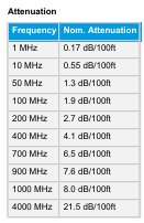
Loss when line is matched is 1,3 dB. Now we will use the ARRL Antenna Book table to compute the additional loss due to SWR:

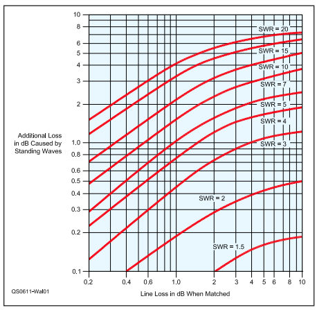
The horizontal scale axis is not linear, is logarithmic. Since 0,3, or 3 dB is the half or the double (depending on the sign), a value of 1,3 is halfway between 1 and 2. Looking at the diagram, you can check that the value of the additional loss caused by the SWR is approximately 0,6 dB.

Let’s now open the HRC and swap the power:

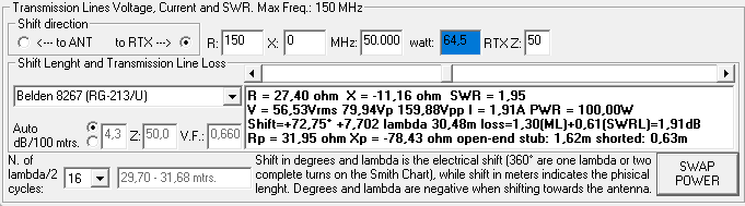
First of all, we notice that the Matched Loss is exactly the one published by Belden, and this is a proof of the HRC database accuracy, so is the computation of the additional loss, coherent with the ARRL Antenna Book table.
At a second glance, we see that this loss reduces the power level of the antenna at 64,5 watt. This is also true, since if you multiply 64,5 by 10 raised to 0,191 (1,91 dB means 10 raised to 0,191) you obtain 100.
Now, SWR is 3, and we know that when SWR is 3, the reflected power is 25% of the forward power, so the antenna reflects 16,1 watt. This reflected power will be attenuated by 1,91 dB too, so the value that will reach the RTX will be 16,1 x 10^(-0,191) which is 10,37 watt. This means that, when the RTX produce 100 watt, the power which is reflected to it is 10,37 watt.
We can now crosscheck the impedance values on the upper left section of HRC and then activate the Auxiliary Data:

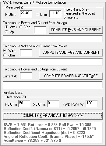
SWR is 1,95, the same computed in the lower section, and reflected power for 100 forward power is 10,39 watt, in accordance with our computation. If you like to double check this with another tool, just take in consideration a common SWR table, with reflected power levels aginst SWR. For an SWR of 2 the reflected power is 11,1% of the forward power. We experienced 10,37%, so our SWR must be slightly less than 2. Results coherence is confirmed again.
You can download an Excel file to perform further computations: www.k0fc.net/content/files/CoherenceCheck.xltx

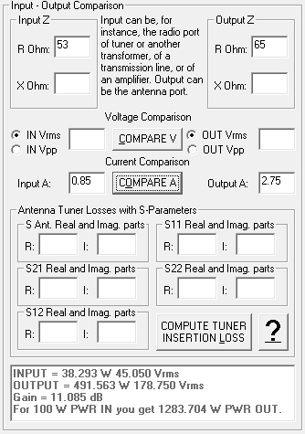
Power level comparison

The HRC right section is dedicated to power comparison computations. It is intended to compare the input and the output power values in a DUT (Device Under Test). The DUT can be an amplifier, in this case HRC will show the gain, or a toroidal transformer, like the 9:1, 49:1, an antenna tuner, or a transmission line, or whatever DUT whose Insertion Loss is the object of our investigation.

We now anticipate that a two-ports VNA is able to compute a DUT Insertion Loss without the need of other instruments, as we will demonstrate later on. We would like to show that HRC is able to have a different approach. Although we could use it to compute an amplifier gain, as we did in pic. 18, in the following pages we will test the power loss computation, once again, on an antenna tuner.

The power meter limitations

There are many fellow hams who still believe that the antenna tuner, when stationary waves are presents, absorbs the reflected power. To disprove this theory, sufficient should be to say that, with 500 W power and an SWR of 6, the reflected power level would be above 250W. The tuner will burn our fingers immediately!
Thinking of power measurements, our mind will probably go to the cross-needles power meter, or to other kind of power meters.
We could install the power meter just before the tuner input port (the RTX side port). Then, once the tuning process is completed, take note of the forward power. The result is shown in the following picture, with the RTX power level set at 10W.

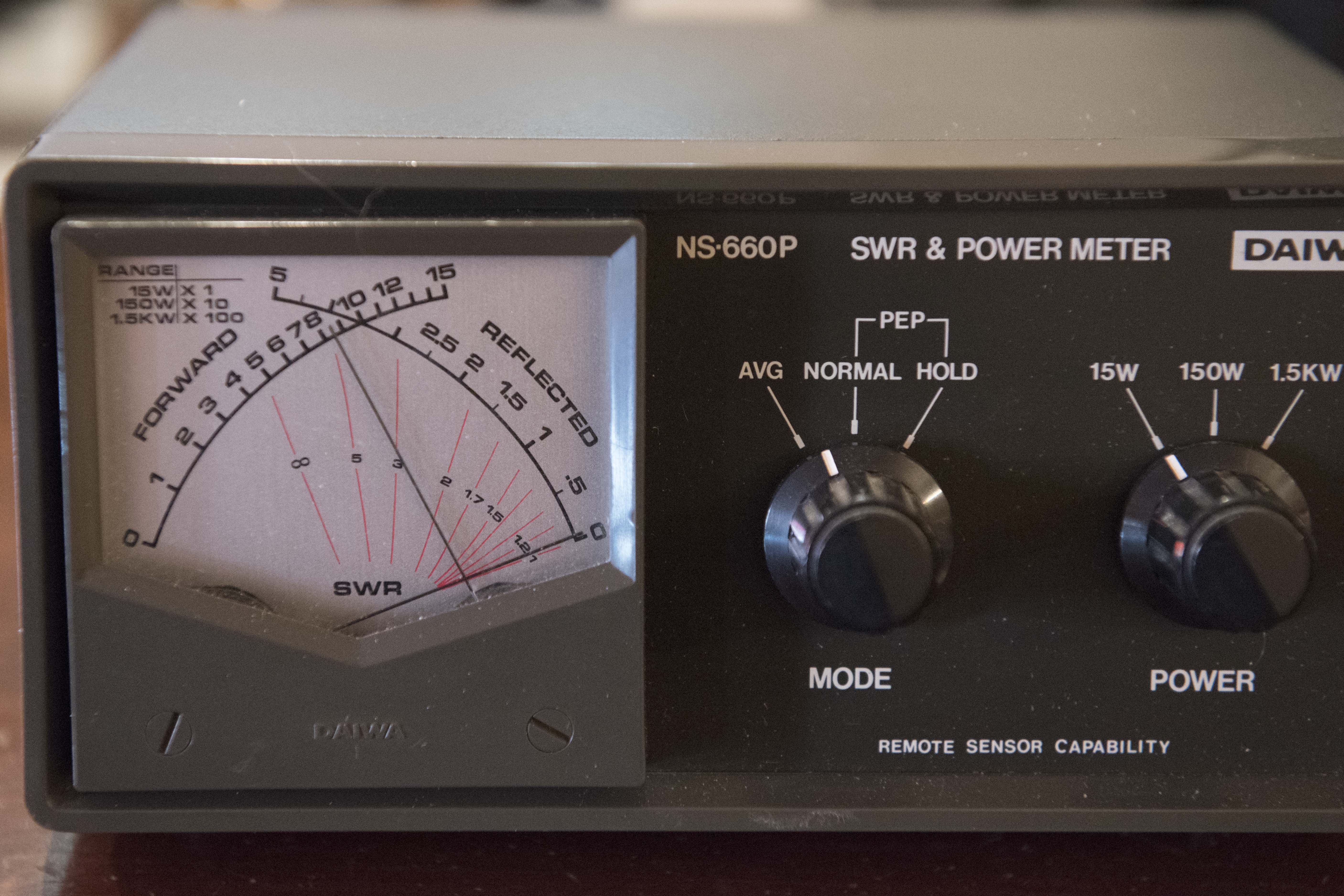
The power meter shows a direct power of 8,5W which is coherent with the RTX level set, since it is often an optimistic value. Reflected power is negligible, which is a sign of a perfect match. Now let’s move the power meter just after the antenna tuner output (ANT) port.

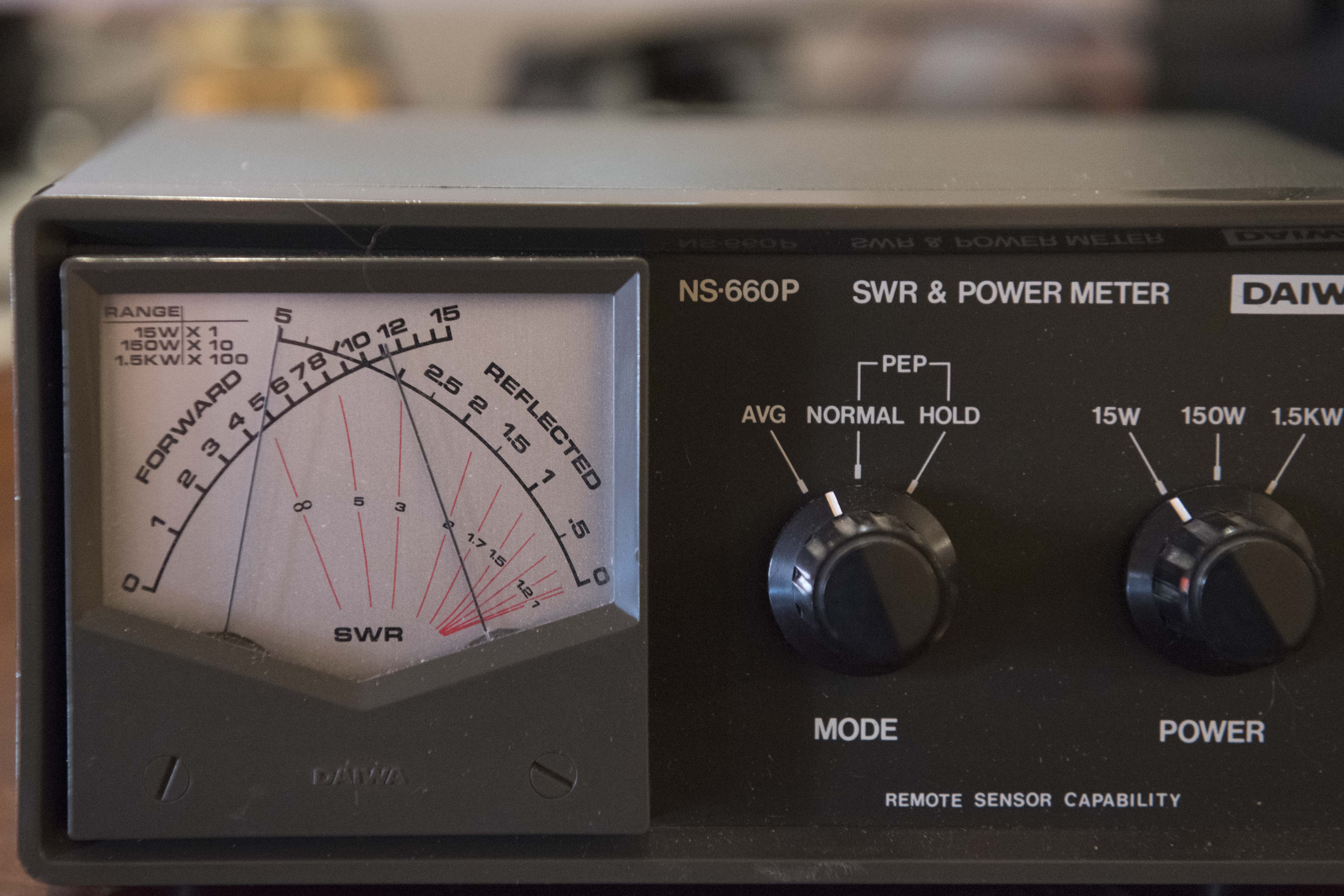
What is the power meter saying? Why, with stationary waves, forward power has grown up? We get more than 11 W of forward power and 5W of reflected power, what happened?
It happened that power exits from the tuner, and part of it is reflected by the antenna. This reflected power, when passing through the tuner, is 5W. Then, it reaches the tuner, and the almost total of it is reflected again towards the antenna, passing, of course, through the meter. A figure of slightly more than 11W is so obtained by the original forward power plus most of the re-reflected power. We can only conclude that, probably, the forward power is in the order of about 7W.

Note: instead of talking about forward and reflected power, which is a widely spread simplified model, we should rather talk about voltage and current waves, and power levels resulting from the interactions of these waves values.
It is now clear that the power meter is a valuable instrument when used for its own purpose only: to show the power on a matched circuit, when reflected power is zero or almost zero. Its place is between the RTX and the tuner, or between the amplifier and the tuner and, even then, it has en error of a few percentage of the full-scale value. The more is the reflected power, the less precise is the power meter. When mismatch is present, you just cannot count on a power meter to compare input and output power.
You noticed I have left the scale on the 15W-5W selection. Although I could have chosen the 150W-50W to check where the needles matched, I wanted to point out that the SWR value is of no importance when comparing the input power with the output one. We will show the impedance and SWR of this case later on.

Exit Ways

We have three other ways to compute input and output power in presence of impedance mismatch. Let’s just apply Ohm’s laws!
This time we need to know the impedance which is present at the point of measurement with the utmost accuracy. As a matter of fact, this impedance will be different from the antenna impedance, since the cable acts as a transformer (after all, a transmission line is an LC circuit, as a tuner). Unless the antenna Z = R + j0 and R is the same as the cable characteristic impedance, as we advance along the cable from the antenna, we will meet different couples of R and X values every time. If the transmission line is a 50 ohm cable, the SWRs of these R and X values will always be the same in respect to 50 ohm. So we will measure Z at the end of the cable coming from the antenna. After that, we will choose between two (initially) chances: check voltage or check current. As we know, Ohm’s laws state that P = V² / Z or P = I² x Z. Once we know Z, with V or I we can compute P.

Measuring impedance and voltage

It is now time to switch our VNA, or antenna analyzer, on.
To measure impedance I used a NanoVna, a very common and accurate device. Since we will perform a one-port measurement, a good antenna analyzer will be sufficient for this purpose.
The proper instrument to measure voltage is, guess what, a voltage meter, or, let’s say it better, an RF voltmeter. But, if you already have an oscilloscope, you can use the latter to measure RF voltage.
Both the Rf voltmeter and the scope have an issue: their probes introduce some capacitance to ground. The solution (not an absolute one) could be a rectifying probes equipped RF voltmeter, but it is an expensive instrument, and it is rare to find a fellow ham who can borrow one.
I used a scope. If you take some precautions you will get acceptable results.
First of all, bandwith should be at least five times the maximum involved frequency. I used a 2 channels scope with 200 MHz bandwith for frequencies up to 21 MHz. Regarding the probes, mine have 350 MHz bandwith, 300V rated voltage and 10 Mohm impedance when selected on 10X.
Do not be impressed by the datasheet: the above values are only valid at low frequencies. As soon as you reach the HF spectrum, those numbers drop drastically. You can think that a 10 Mohm impedance induces a negligible impact on the measurements. Well, at 1 MHz the impedance is already a few hundreds ohm, while rated voltage is 25-30V.
So, let’s go back to the HRC left section, enter the minimum power that your RTX can be selected on, and check against the impedance to see which voltage you can expect. If the value is near the rated probe value for the frequency in use, just put an attenuator on the RTX. I would suggest a 20 dB attenuation, since resulting voltages will be ten times smaller, making computations easier.
The other precaution is to measure the impedance with probes connected and scope on (and RTX off!), so we will use the updated impedance, the one disturbed by the probes, which is exactly the Z we have to check.
Let’s see now how to realize this measurement.

We have to arrange a fixture so as to measure impedance and voltage on the same place.
The first action is to perform the calibration on the VNA. We generally comply the calibration with three male connectors, which actually are calibration standards, named Short, Open, Load. They are mounted on a female barrel socket at the end of a short cable coming from the VNA (or analyzer). Now, the trick is to prepare the cable coming from the antenna with a similar socket, entering into a T-shaped adapter. The opposite side of the T will go to the tuner, so we have the central port of the T available for the scope probe.

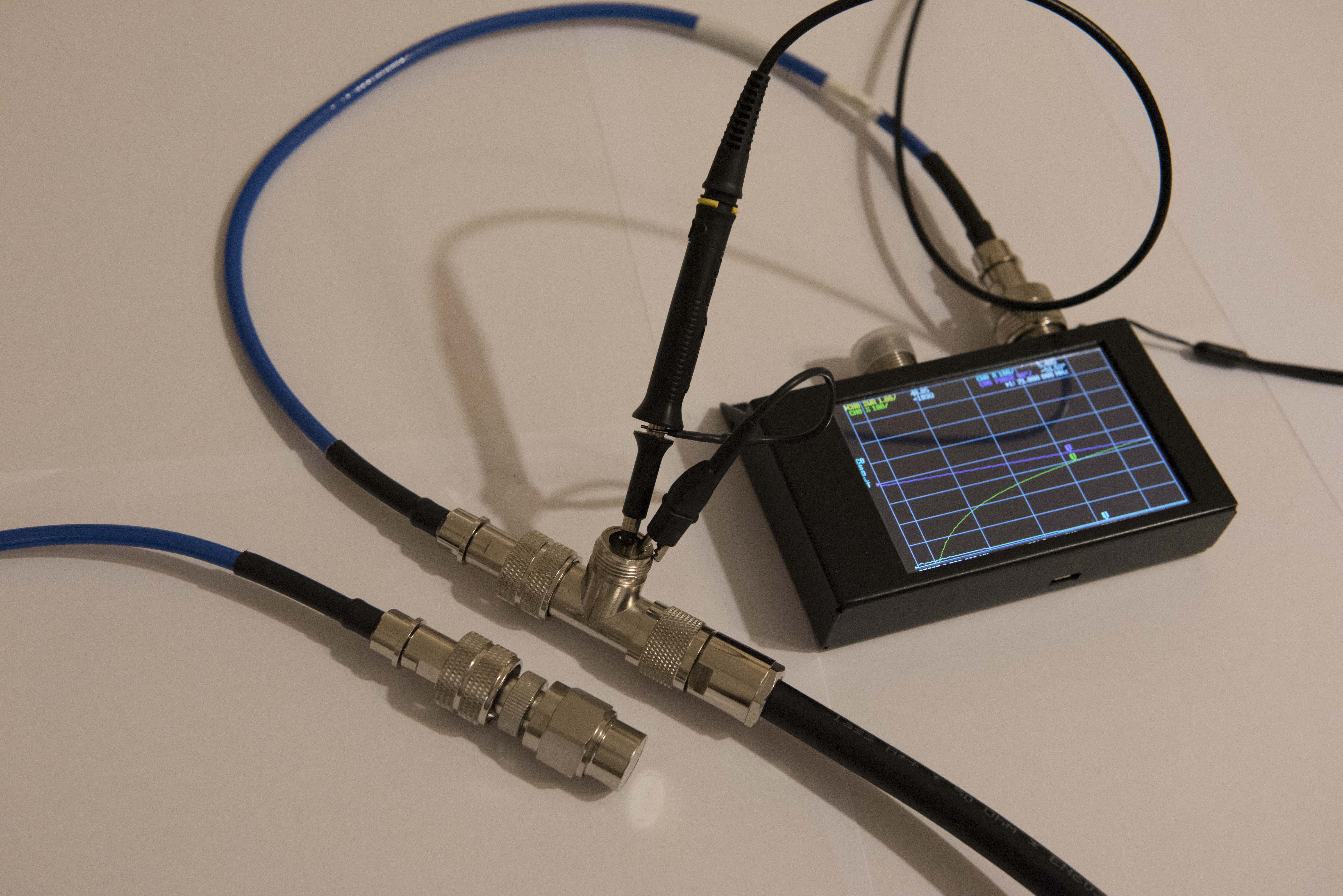
Please check picture 21. I assembled a calibration standard on a female barrel connected to a cable. As reference you see the fixture I just described. It is evident that probes are very close, if not exactly, where you measure the impedance.

The following is a step by step guide to perform a valuable voltage measurement:

Insert the cable from the VNA into the T-shaped adapter as shown in the picture (with this arrangement the calibration standard reference plane lies very close, if not exactly, where the probe reads the voltage). Connect the probe to the T center port. On the remaining port connect the cable from the antenna. Switch the scope on, set the probe at 10X and read Z on the VNA. In our case, R = 10,8 ohm, X = 12,4 ohm at an operating frequency of 21 MHz.
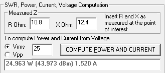
Compute, with the HRC left section, at which power level you reach the maximum safe voltage for the probe. In our example, I wanted to be sure voltage did not exceed 25Vrms, so the maximum power to be used was 25W (look at the picture above).
If R is high you can reach hazardous voltages for the probe with even less than 5W. If this is the case, use an attenuator at the RTX output. With a 20 dB attenuation voltage are ten times lower, with 40 dB one hundred times lower.
Remove the VNA from the fixture, and connect the shortest possible cable to the tuner (ANT port) in its place.
Arrange a similar fixture on the other side of the tuner, one side of the T-shaped adaptor to the RTX and the other, with the shortest possible cable, to the tuner (RTX port).
To preserve the scope, disconnect momentarily the probes on both fixture, and tune, as you are used to do, the antenna tuner. The reason is, while tuning (especially with fast switching relays, as in automatic tuners) you can experience very harmful voltage for the scope.
Reconnect the probes once the tuning process is completed. This will slightly vary the tuning. It is not a problem: we are interested in coherence between voltage against impedance measurement. Once we get the voltage measurement with the impedance corrected for the probes (which is our case) we are fine. The small mismatch that will result does not bother the input-output power comparison.
Momentarily disconnect the cable from the RTX and connect in its place the calibrated cable from the VNA. Reconnect the probes and check the impedance on the VNA, with the scope on. In our case R = 50,2 and X = 5,5 ohm.
Repeat the previous procedure to check the maximum power we can use without exceeding 25 V, this time with Z = 50,2 + j5,5. This time the HRC shows 12 W. To perform a safe measurement we decide to use 10 W, in order not to overcome the probes rating on both sides of the tuner.
Disconnect the VNA and reconnect the RTX.
Transmit a 10W CW note.

Take note of the oscilloscope measured voltage values. I set channel 1, yellow, on the output and channel 2, blue, on the input. This is the result.

Above we have the voltage at input and output: 22,2Vrms and 14,9Vrms respectively. The signal has traveled for 8 nanoseconds from the first point of measurement to the second one.
Now that we have all the necessary data we can enter their values:

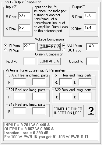
The lower window shows us that input power was 9.7W, output power 8.9W, the insertion loss about 0.4 dB. This means that if you send 100W to the tuner, 91W will exit from it.
These results are worth some considerations. First of all, we obtained them with two instruments. I am positive my NanoVna SAA-2N (2.2) is, at least in the HF spectrum, accurate. Anyway I did not check its results against a professional laboratory grade instrument. About the scope, which shows its results in a magnificent way, we already know it has some deviations, even if we adopted a strategy to reduce them at the minimum possible level. Now, did the (possible) VNA deviations and the (certain) scope deviations compensate each other, or did they sum up? We do not know. Are the two figures approximated down or up? Still, we do not know. So it is nonsense to compare third decimal order figures, but, out of the fog, a figure is clear: our antenna tuner, at least on the checked frequency and impedance, shows a very low insertion loss, at least lower than many hams would swear on: around one half dB, or, in percentage, around 10%.

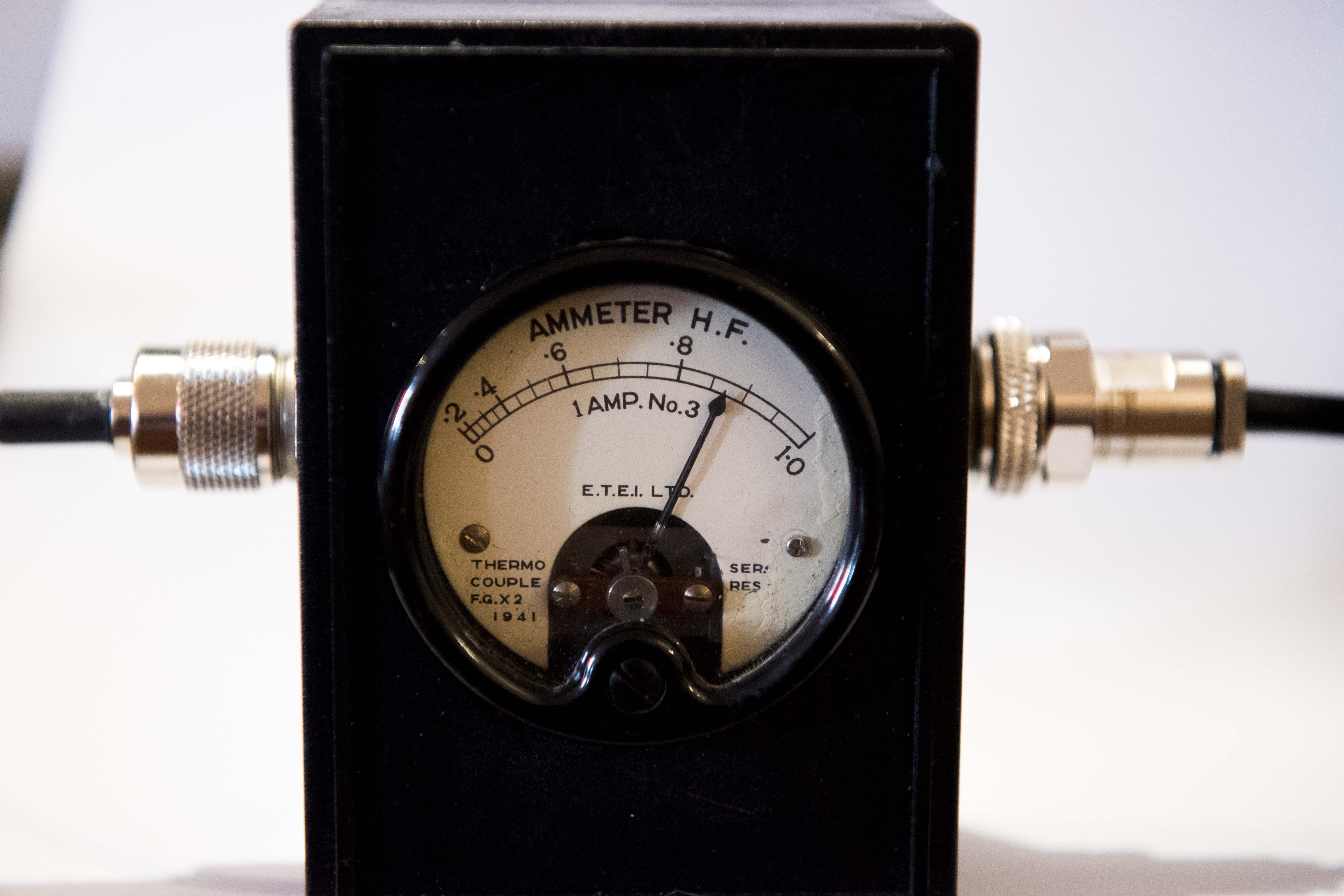
Measuring Current

To measure the current we need, guess again, an ammeter, but since we are measuring RF, we decided to name it, what a fantasy, RF ammeter.
The Rf ammeter is a straight instrument, affordable, lightweight and, most of all, reliable. Should I have presented you the current measurement before, you would have jumped the voltage section, for sure!
I have used a vintage device, thermocouple based, which is a gift from a fellow ham, Antonio I0JX. Due to its nature, you have to wait a few seconds to get the final figure, but it is accurate and, as I said before, reliable.
You can buy a new one, from ham radio accessory manufacturers, or you can also find a good used one on the bay. Your choice.
My Rf ammeter is 1A rated. Once again, we will use the left HRC section to check a safe power level in order to not exceed a 1A current, based on the impedance.

Current measurements are far more practical than voltage measurements to realize, since we do not need any special fixture to arrange anymore. We just need some adapters to mount the RF ammeter alternatively, once on the input and once on the output side.
As before, the first step is measure the impedance and check the maximum safe power level.
This time, impedance is a little different. This is due to the lack of the probes influence: we get R = 49,5 and X = 5,4 ohm at input, R = 10,5 and X = 12,1 ohm at output.
Note: to compute power from current, the reactance value is useless, so, as you will see in the next picture, we left the windows void, since HRC will not process the entered values at all.
Then, we check the proper power level to use. We can try to enter 10W, to have the same power reference as before (actually, you do not need this value to be the same) on the left section and see the results: I will not show them, you now master the HRC. Anyway, we expect a little less than 0,5A at input and less than 1A at output, so we will proceed with 10 W from the RTX. And the results are: 0,42A at input and 0,87A at output.
As we did for voltage, we enter these values, together with the impedance ones, on the HRC:

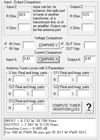
Results, a little lower in absolute level in respect to the ones obtained by means of voltages, are surprisingly (well, we shouldn’t be surprised) similar, when considering the comparison level, to the results obtained with the oscilloscope. An insertion loss of about one half dB, or 10%, is completely confirmed.

Half... final considerations

We already discussed the voltage comparison results. Current comparison has been a confirmation.
It’ is not an antenna tuner “Road Test”, nor was intended to be. A complete tuner test should take in consideration more frequencies and more type of impedance, as low or high resistance, positive or negative reactance. We just wanted to point out that the antenna tuner insertion loss is not the one many ham consider.
Most of all, we acquired a methodology to evaluate voltage and current values involved in our devices, in order to be more aware of our operating conditions, if they are safe or potentially harmful.

Saving the best for last: VNA-only power comparison

Let’s see now the most accurate method to compute an antenna tuner insertion loss: we are talking about the VNA only computation. Here a single instrument is involved, without suffering the capacitance effect of the probes, and we are using this instrument accordingly to the purpose it has been created for: voltage wave measurements.
From now on, for VNA we intend a two-port VNA, a simple one-port antenna analyzer is no more sufficient.
The VNA is an instrument that emits an RF signal towards a device to be measured, the so called DUT (Device Under Test), an antenna tuner (again!) in our case. It will measure both the DUT reflected signal and the signal that has crossed the DUT itself. Since a voltage wave is a vector, it must be expressed with two numbers. So we have to treat these numbers accordingly to the complex number algebra. A complex number is a number formed by two parts, a real one and an imaginary one. Complex numbers fit perfectly the need to represent impedance values and voltage wave values.
The VNA first port is generally called TX, or Port 1, the second port RX, or Port 2. The popular NanoVna has different names: Port 1 is also called Channel 0 (CH 0), while Port 2 is also called Channel 1 (CH1). So, please pay attention!

To evaluate the tuner insertion loss, we will compare the wave from the VNA to the tuner and the wave exiting from it. Actually, the computing is not so straightforward, since reflections from the antenna and back from the tuner to the antenna are involved. Moreover, the only S₂₁ reading is not sufficient to compute the tuner insertion loss, because at least one of the two tuner ports impedance is not 50 + J0 ohm.
These are the steps to be followed:

Perform the SOLT calibration; VNA calibration procedure is quite straightforward, but varies from model to model, it is beyond this guide’s purpose to explain it in details.
Connect the cable coming from port 1 to the transmission line coming from the antenna (a barrel female-female adapter might be needed). Port 2 will remain disconnected. Read the S₁₁ real part and the imaginary part value on the VNA, and insert these two values as the real and the imaginary part of the “S. Ant.” windows. S_xx parameters may be showed in different formats. We will choose the one which gives the real and the imaginary part directly, but the format name may vary from a VNA manufacturer to another. Consider that S_xx parameters are dimensionless complex numbers. Further on, I will give detailed instructions for the NanoVna.
Put the tuner on line, that is, connect the tuner ANT port to the transmission line coming from the antenna. Connect the tuner RTX port to the cable coming from the VNA Port 1. Port 2 remains disconnected. Start the tuning process with the aid of the VNA (using always the same calibration), reaching the lowest possible SWR, 1 if feasible.
Remove the transmission line, and connect (with the same cable used in the calibration process) the tuner ANT port to the VNA port 2. The tuner RTX port remains connected to the VNA Port 1. Read on the VNA the S₁₁ and the S₂₁ parameters, and insert them into the respective HRC windows.
Swap the ports: cable from VNA Port 1 shall be connected to the tuner ANT port, while the cable coming from VNA Port 2 will go to the tuner RTX port. Read the S₁₁ and S₂₁ parameters on the VNA. This time insert the S₁₁ parameters into the HRC S₂₂ windows, and the S₂₁ parameters into the S₁₂ HRC windows.
If the tuner has no ferrite element in it, it is likely that S₂₁ = S₁₂. That is the reason why, when you enter a value in the S₂₁ window, the S₁₂ window will be automatically updated. Of course, you can change the S₁₂ parameters without changing S₂₁. So, to avoid mistakes, always follow the proposed order to enter the S_xx parameters in the HRC.
It is of the utmost importance to use the same calibration and cables during all the measuring process.
All the HRC windows related to S_xx parameters contain a ToolTip label: positioning the mouse over a window the ToolTip level will popup, remembering the right action to perform.

Note: as already pointed out, S₂₁ only reading is not sufficient to compute the tuner loss, because the antenna port impedance is not 50 + J0 ohm.

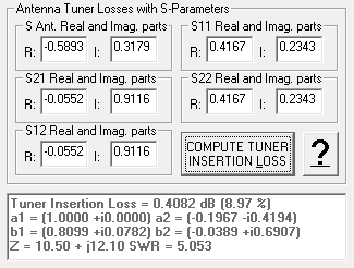
In the above picture you have an example of VNA-Only loss computation. Besides the insertion loss value in dB and percentage, HRC shows the four voltage waves a1, a2, b1 and b2 values. a1 voltage wave is the fixed reference for the input power, so its value is 1+i0, a2 is the antenna reflected wave, b1 the reflected wave by the tuner towards the RTX, b2 is the antenna reflected wave that, upon reaching the tuner, is reflected again toward the antenna. The window presents the impedance related to the S. Ant. inserted and the resulting SWR.

With the described measuring process (as in the voltage and current cases) you evaluate the insertion loss of the tuner. The additional loss caused by the remaining SWR (if any) between the RTX and the tuner will not be computed.

NanoVna directions

I will now give a guide to obtain the S_xx parameters in the correct format with the NanoVna, at least with the present firmware.
It is advisable to save the proper format before calibration, so as to have it ready anytime you recall the calibration itself. Anyway the format, if convenient, can be changed at any moment without affecting the calibration.
From the main page choose DISPLAY from the menu, then TRACE, and you have the choice to select one among trace 0, 1, 2, or 3. Let’s start with 0, after having selected it we go to BACK, then CHANNEL, and select CH0 REFLECT, then BACK, FORMAT, SWR and exit menu. In this way we have instructed the NanoVna to show the SWR value on the Trace 0. This will be useful in the tuning process.
Enter the menu again, select TRACE 1, BACK, CHANNEL, CH0 REFLECT, BACK, FORMAT, MORE, POLAR and exit the menu. Trace 1 will show two values side by side. They are the real part and the imaginary part of an S_xx parameter, as registered by Port 1 (CH0) parameter.
Enter the menu again, select TRACE 2, then BACK, CHANNEL, CH1 THROUGH, BACK, FORMAT, MORE, POLAR and exit the menu. Trace 2 will show the Sxx parameters as Trace 1, but this time associated to Port 2 (CH1).
For step 2) of the previous paragraph please read Trace 1, entering the real and the imaginary figures in the respective HRC “S. Ant.” windows.
For step 3) you can tune with the Trace 0 SWR indications.
For step 4) please read the S₁₁ real and the imaginary part on Trace 1, and the S₂₁ ones on Trace 2. As already said, the S₂₁ and S₁₂ values may coincide.
Steps 5), 6) and 7) recommendations remain valid.

An example of tuner comparison

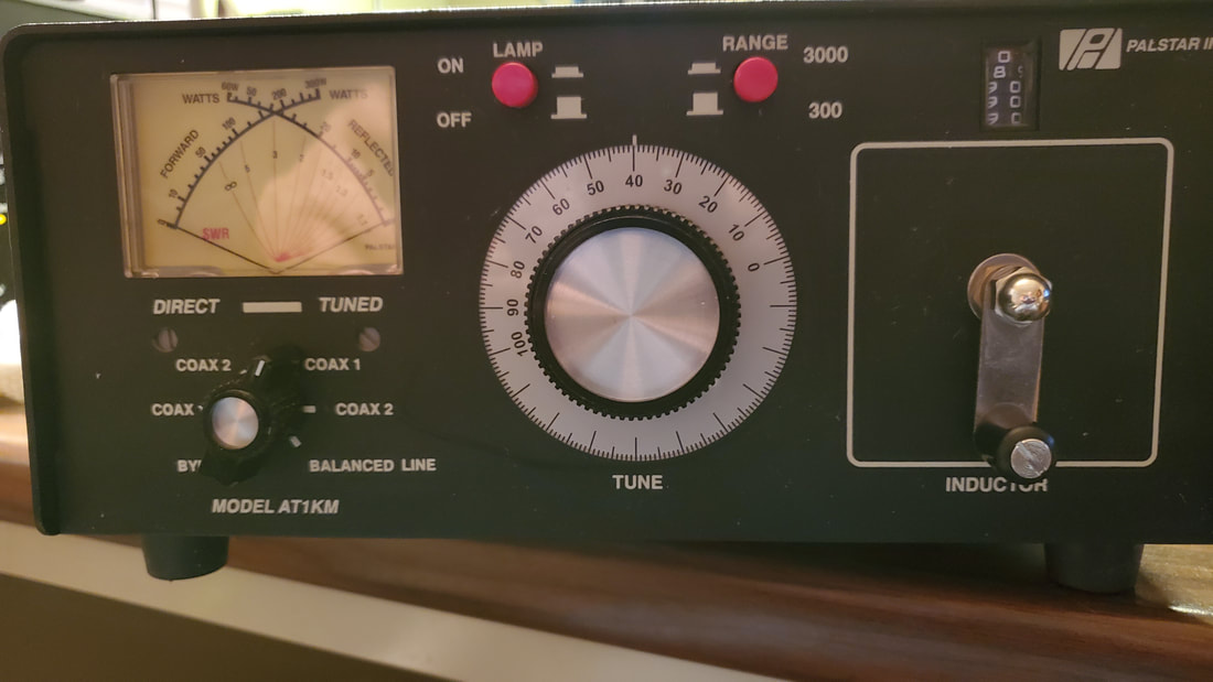
Let’s now make an efficiency comparison between two tuners, the Palstar AT1KM (T tuner with two capacitors commanded by a single axis and roller inductor),

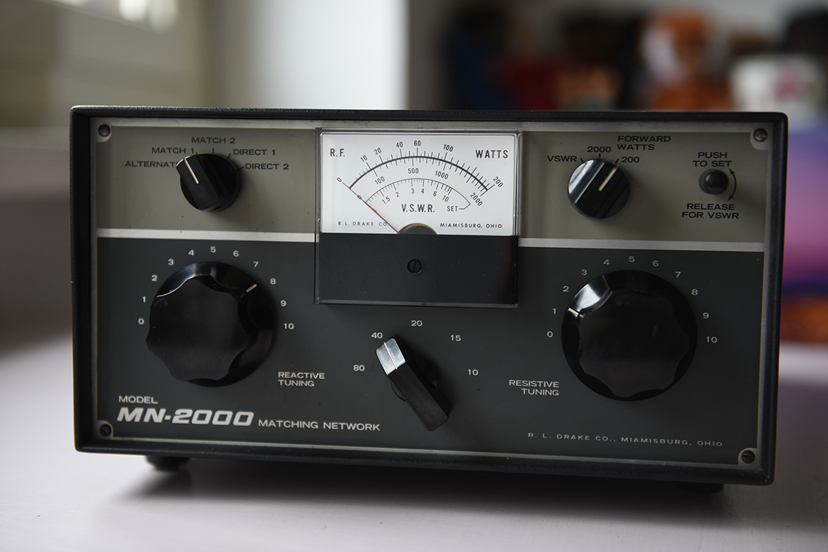
and the Drake MN-2000 (greek PI tuner, rotatory switch inductor).

They share one characteristic: there is only one possible configuration to obtain the best match. The antenna is the same, the impedance at the RTX end of the cable is approximately R = 74 and X = 110, SWR = 5,3. Both tuners reached an SWR of 1 after tuning. Measures were performed with a VNWA 3 by DG8SAQ:

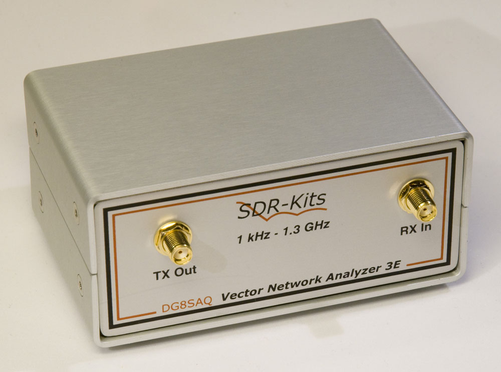
Here are the results:

Palstar:

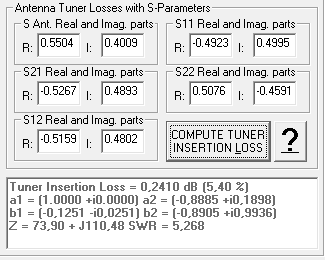
Drake:

Please disregard the a1, a2, b1 and b2 values of the scattering matrix, and just read the insertion loss. It is about 5% for both.
A comprehensive comparison should include measurements of all kind of impedance, with low and high resistances, inductive and capacitive reactances, but it is beyond the purposes of this guide.

Credits

A special thank to Professor Michele D’Amico IZ2EAS, University “Politecnico
di Milano”, for the priceless support in solving the scattering matrix.

Ing. Antonio Vernucci I0JX for his ideas, experience and generosity.

Professor Thomas Baier DG8SAQ, VNWA father, for the precious suggestions.

My daughter Sara, for the present user guide translation. I am so proud of her.

Last update: july 24th, 2025

Homepage

Download HRC 3.1

Download HRC 3.1 (version to be used when MSSTDFMT.dll class is not registered)

Download HRC Guide

Biography

Contacts